It has been a while since I last wrote an article here, and this gap ended up being a little longer than I expected. There was quite a lot I needed to prepare outside the article itself, and my day job has been especially busy lately. I did not want to publish something rushed just to fill the gap, so I kept this project on the side until I had enough time to build it, test it, break it, and measure it properly. The result brings together several things I really enjoy working with: Windows systems programming, computer vision, game control, and reinforcement learning.
Introduction
This project asks a deliberately awkward reinforcement-learning question: can I train a useful controller for an ordinary Windows game without reading its process memory, injecting a DLL, or adding a training API to the game? I use a small Direct3D 11 arena game, SpaceProx.exe, as an external black box. The agent captures the rendered client area with the Windows API, extracts visual geometry from those pixels, chooses actions with a neural actor-critic policy, and controls the executable through ordinary keyboard and mouse input.
The final system is intentionally hybrid rather than pretending that a few thousand real-time interactions are enough to reproduce large-scale end-to-end visual RL. Deterministic computer vision acts as the perception and low-level combat layer; PPO learns the nine-way movement policy. Visible targets are translated into target selection, motion estimation, an intercept calculation, ordinary cursor movement, and firing without accessing hidden game state. The learned observation also includes eight rendered-pixel free-space rays so walls are observable before a movement action repeatedly collides with them. This division lets scarce RL samples focus on navigation and survival instead of relearning target geometry.
Schulman et al. (2017) proposed Proximal Policy Optimization (PPO), while Schulman, Moritz, et al. (2015) introduced Generalized Advantage Estimation (GAE). This implementation uses both, together with a shared neural feature extractor, separate actor and critic branches, PyTorch, per-optimizer-epoch logging, and explicit checkpoint accounting. The article derives the return, value function, TD residual, GAE, policy-gradient objective, PPO probability ratio, clipped surrogate loss, critic loss, entropy term, and gradient update rather than treating PPO as a black box itself.
The implementation also records the engineering failures that matter in a real Windows environment: screenshot resource cleanup, cursor-control failures, delayed title telemetry, episode reset behavior, partial PPO rollouts, policy entropy, and the difference between a model's recorded timestep counter and the transitions that actually reached an optimizer update. Results in this article are taken only from saved logs and evaluation runs; unmeasured performance is not filled in from memory or intuition.
1. Why build RL around a normal executable?
Most RL tutorials start with an environment that already exposes a clean interface:
observation, reward, terminated, truncated, info = env.step(action)That is convenient, but it hides an interesting systems problem. A normal Windows game does not expose a Python step() function. It renders pixels, reads input, updates itself on its own clock, and has no reason to cooperate with an RL library.
I wanted the boundary to look much closer to a human-computer interaction loop than to a simulator-specific API. The game and learner are separate programs, and the runtime boundary is rendered pixels in one direction and ordinary Windows input in the other.
The game
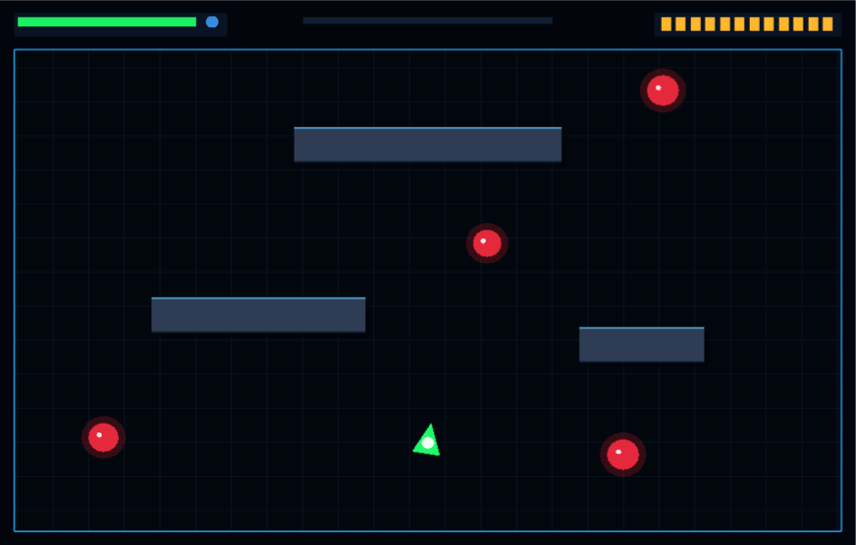
SpaceProx is a small top-down D3D11 arena game. The green triangle is the player, red circles are enemies, and the blue-gray rectangles are walls. The player moves with WASD, aims with the mouse, and fires with Space. Enemies move around the arena, the player loses HP on contact, and the score increases when enemies are destroyed.
The project is split into the standalone game and the external RL controller:
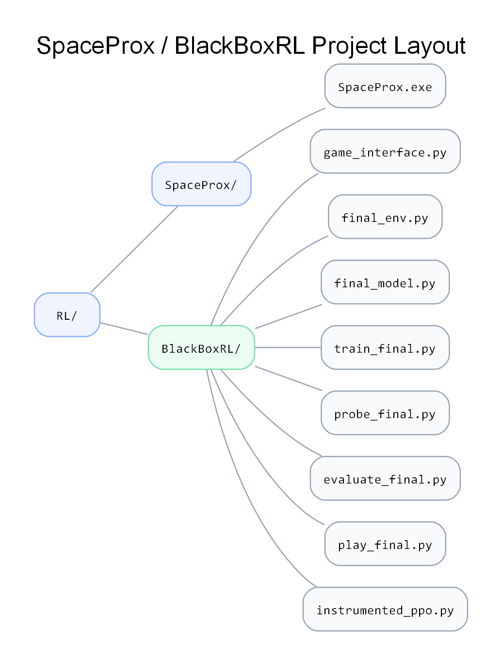
The RL side does not use ReadProcessMemory, pointer offsets, DLL injection, an internal entity list, or a game-engine callback. The title bar is used as external training telemetry for score, HP, and episode state; the deployed policy state is constructed from rendered-pixel measurements together with a short wrapper-maintained motion/history signal and the previous movement action.
This is not the only possible definition of "black box," so I make the boundary explicit instead of hiding it behind a slogan.
2. Research Context and Related Work
The idea of learning game control from interaction is much older and much larger than this project. Bellemare et al. (2013) introduced the Arcade Learning Environment (ALE) as a reproducible platform for evaluating general agents. Mnih et al. (2013) then demonstrated deep Q-learning from game pixels, and the later Nature paper by Mnih et al. (2015) reported human-level control across a suite of Atari games. Mnih et al. (2016) showed an actor-critic route with A3C and emphasized parallel experience collection. Hessel et al. (2018) later combined several major DQN improvements in Rainbow, while Badia et al. (2020) extended exploration far enough for Agent57 to exceed the standard human benchmark across all 57 Atari games.
The sample-efficiency problem remains central. Laskin et al. (2020) proposed CURL, Kostrikov, Yarats, and Fergus (2020) showed how simple image augmentation can regularize pixel-based RL, and Yarats et al. (2021) developed DrQ-v2. World-model approaches provide another route (Ha and Schmidhuber, 2018; Hafner et al., 2021; Hafner et al., 2025), while Sekar et al. (2020) studied self-supervised exploration. These papers are particularly relevant here because experience is the expensive resource: this environment is not a fast simulator running thousands of copies. It is one actual Windows process advancing in real time while Python captures the window and sends OS input.
Large competitive-game systems make the scale mismatch even more obvious. Berner et al. (2019) describe how OpenAI Five used PPO/GAE at enormous distributed throughput and trained for months. Vinyals et al. (2019) combined supervised learning, multi-agent RL, and league training for AlphaStar. Jaderberg et al. (2019) likewise relied on large-scale population-based training in Quake III. From a systems perspective, IMPALA (Espeholt et al., 2018) and Sample Factory (Petrenko et al., 2020) show how aggressively modern RL pipelines try to increase actor throughput. Those systems are inspiration, not fair numerical baselines for a laptop experiment. If anything, their scale is an argument against pretending that a few minutes of single-instance raw-pixel PPO should automatically discover robust perception, aiming, navigation, and credit assignment at once.
That leads to the design decision that shaped this project: keep the executable black-box, but do not force the neural policy to relearn deterministic geometry that can be recovered reliably from the same pixels. Sutton, Precup, and Singh (1999) formalized temporal abstraction through options. Bacon, Harb, and Precup (2017) later developed Option-Critic, while Kulkarni et al. (2016) and Vezhnevets et al. (2017) explored hierarchical deep-RL architectures. My implementation is simpler than those methods. It uses an engineered low-level controller, but the motivation is related: learn the decision that matters at the higher level and delegate mechanically solvable control to a lower layer.
This distinction also makes the scientific claim narrower and more defensible. The final system is a hybrid visual RL controller, not a claim of general end-to-end representation learning from raw pixels.
3. Experimental constraints
The constraints are part of the experiment, not incidental implementation details.
| Constraint | Choice in this project |
|---|---|
| Game access | external executable only |
| Internal memory | not read |
| Injection/hooks | not used by the RL runtime |
| Visual sensing | Win32 PrintWindow client capture |
| Policy state | rendered-pixel features + short history + previous movement action |
| Reward telemetry | score/HP/state already exposed in the public window title |
| Control | ordinary Windows keyboard and cursor input |
| Learning | PPO + GAE |
| Hardware | NVIDIA RTX 4060 Laptop GPU |
| Framework | PyTorch + Stable-Baselines3 |
| Parallel environments | one real game instance during a valid run |
The single-environment constraint is especially important. Parallel actors are a standard way to make deep RL practical (Mnih et al., 2016), while distributed agents such as IMPALA separate acting and learning at enormous scale. Here, every fresh transition costs actual wall-clock time. A bad observation/action design is therefore far more expensive than it would be in a cheap simulator.
4. System architecture
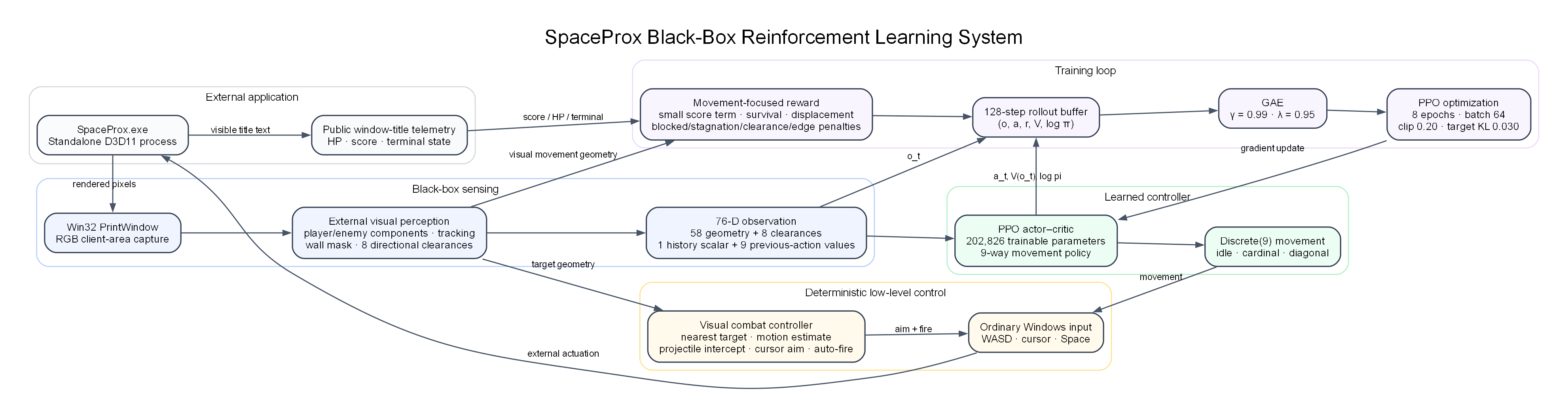
The final controller is organized as a closed external control loop around SpaceProx.exe. Rendering, perception, learned movement, low-level combat control, reward construction and PPO optimization are shown together below.
There are two separate feedback channels:
- Policy observation: geometry derived from the current rendered frame.
- Teacher/evaluation signal: public title telemetry supplies exact score and HP
deltas and confirms the episode boundary.
The policy is not given process-memory coordinates or an enemy array. The apparent coordinates it receives are measurements made by the perception code from the captured image.
5. Capturing the game window
Capturing the full desktop is a surprisingly bad RL sensor. A training terminal can cover the game, notifications can appear, the taskbar can move, and another window can become the accidental observation.
Instead I locate the game HWND and capture its client area directly:
ok = ctypes.windll.user32.PrintWindow(
    hwnd,
    memory_dc.GetSafeHdc(),
    3,
)
The returned bitmap is BGRA, which I convert to RGB. The capture code also has to manage GDI resources correctly. During long experiments I observed occasional cleanup errors even after a successful frame capture. Cleanup therefore happens in finally, but release failures are not allowed to retroactively invalidate an otherwise valid observation.
That sounds like boring Windows plumbing. It is also part of the RL experiment: one bad screenshot path can make the policy blind while the optimizer continues printing perfectly respectable-looking losses.
6. Computer vision as an external sensor, not hidden state
The rendered game intentionally uses strong colors. The player is bright green; normal enemies are red. Instead of discarding that signal, the final perception front-end uses it.
6.1. Player detection
The first stage thresholds pixels where green strongly dominates red and blue:
green = (
    (g > 175)
    & (g > r * 1.55)
    & (g > b * 1.35)
    & (r < 150)
)
The HUD is also partly green, so the top strip is excluded. Connected-component analysis rejects small noise and keeps the player-sized component. Inside that component I search for the small bright center disk, which gives a more stable center estimate than taking the median of a triangle whose visible pixels change when it rotates.
6.2. Enemy detection
Enemy bodies are detected with the complementary red-dominant mask, followed by component area and bounding-box filters. Importantly, the system only sees enemies that the game actually renders. It does not recover an internal enemy that is hidden behind geometry.
6.3. Why a GAME OVER detector is useful
The title is refreshed more slowly than the environment step. That creates a short window in which the rendered frame already shows GAME OVER while the title can still contain the previous HP/state text.
I therefore detect the dark screen plus red border visually. This gives immediate episode termination and avoids training on one to three dead-screen transitions while waiting for text telemetry to catch up.
6.4. Tracking motion without identity labels
The wrapper never receives an enemy ID. It estimates short-term motion by greedily matching each current red component to the nearest unmatched component in the previous frame. At the game's speed and an 80 ms environment interval, the expected inter-frame displacement is small enough that a conservative distance gate works well for visible enemies.
For an enemy center matched to :
and the screen-space velocity estimate is approximately:
This is still black-box sensing. It is the same kind of inference a vision system would make from two camera frames.
7. Why target aiming is a low-level controller
At first glance it sounds more "pure" to ask PPO to output an aim sector directly. For this real-time experiment that is mostly a sample-efficiency tax. The policy would have to learn all of the following indirectly from reward:
- which colored object is an enemy;
- where the player is;
- the relative angle between them;
- how an integer action maps to a mouse direction;
- how much to lead a moving target;
- that firing is only useful when the aim is sensible.
None of those is the strategic decision I care about. They are geometry.
So the low-level controller chooses the nearest visible target and computes an intercept point. Let the vector from player to target be , target velocity be , projectile speed be , and interception time be . Interception requires:
Squaring both sides gives:
which is a quadratic in . I take the smallest positive solution when one exists, clamp unreasonable prediction horizons, and aim the ordinary Windows cursor at:
If tracking is insufficient, the controller falls back to direct aim.
This is not an Option-Critic implementation. Bacon, Harb, and Precup (2017) learn options and their termination behavior, whereas the low-level controller here is engineered explicitly. Sutton, Precup, and Singh (1999) provide the broader temporal abstraction framework, and later hierarchical deep-RL work by Kulkarni et al. (2016) and Vezhnevets et al. (2017) illustrates related ways to reduce the effective decision space. The visual-control side has a different lineage. Hutchinson, Hager, and Corke (1996) describe classical visual servoing, where image measurements close a real-time control loop. Levine et al. (2016) demonstrate the opposite design point, learning perception and control jointly. I use the hybrid boundary here because the interaction budget is tiny by deep-RL standards.
8. The learned action space
The learned action is deliberately narrow: PPO chooses only one of the nine movement commands already available to a human player:
movement:
0  idle
1  W
2  S
3  A
4  D
5  W+A
6  W+D
7  S+A
8  S+D
When a valid rendered enemy exists, the low-level visual controller automatically aims and fires. That choice is intentional: in this game, with no friendly-fire penalty and an automatic reload after the magazine empties, refusing to shoot a valid visible target was not the strategic behavior I wanted PPO to spend its tiny interaction budget discovering. The learned problem is therefore Discrete(9) navigation while combat execution is a deterministic visual-control subtask.
The maximum policy entropy is now:
which is also a convenient sanity check for training logs.
9. The 76-dimensional visual state
The learned policy receives 76 floating-point features, all derived from rendered pixels, the immediately preceding frame, or the previous movement action.
Player and Arena Features (9 values)
normalized player x
normalized player y
player-present flag
normalized player delta-x
normalized player delta-y
left-edge proximity
right-edge proximity
top-edge proximity
bottom-edge proximity
Nearest Target Summary (7 values)
visible enemy count / 7
nearest target relative x
nearest target relative y
nearest target distance
nearest target delta-x
nearest target delta-y
nearest target present flag
Per-Enemy Slots (42 values)
Up to seven visible enemies are sorted by distance from the player. Each contributes:
relative x
relative y
distance
delta-x
delta-y
present flag
so:
The original visual geometry therefore contributes:
Missing enemy slots are zero-filled.
Directional Wall Clearance (8 values)
A failure mode exposed by deterministic playback was especially instructive: a nearly uniform policy could choose W by a tiny logit margin and then keep pressing it against an internal wall. Player/enemy geometry alone did not tell the network which movement directions were immediately obstructed.
The final state therefore ray-casts through a wall mask built from the rendered blue-gray obstacle pixels. One normalized free-space value is produced for each non-idle movement direction:
W, S, A, D, W+A, W+D, S+A, S+DThe obstacle mask is dilated by approximately the player's visual/collision radius, so a ray estimates whether the body can move through the direction rather than whether one mathematical center pixel is free. No wall coordinates are read from game memory.
Recent Behavior (10 values)
One scalar summarizes the spatial extent of recent player positions and a 9-way one-hot vector records the previous movement action. The history signal helps distinguish useful sustained travel from repeatedly issuing a command that produces little displacement.
The complete dimensionality is therefore:
This representation is a deliberate engineering trade-off. DQN showed that deep RL can learn representations directly from pixels (Mnih et al., 2013; Mnih et al., 2015), and modern visual-RL work has made that dramatically more data-efficient (Laskin et al., 2020; Kostrikov, Yarats, and Fergus, 2020; Yarats et al., 2021; Hafner et al., 2025). But those results do not imply that raw-pixel PPO is automatically the right choice for an eight-frames-per-second single-process experiment. The final controller spends its scarce RL samples on control rather than rediscovering a color segmentation problem.
10. MDP or POMDP?
An MDP assumes the current state contains everything needed to predict what happens next. A POMDP is the more realistic case here: the controller sees an observation, not every hidden variable inside the game.
Sutton and Barto (2018) give the standard reinforcement-learning formulation in terms of states, actions, transitions, rewards, and discounted return. In that notation, an MDP is commonly written as:
where is the state space, the action space, the transition dynamics, the reward function, and the discount factor.
The neural policy does not observe the game's true internal state. Enemy respawn timers, projectile lifetimes, cooldowns, collision state, and hidden variables remain inside the executable. The controller sees an observation constructed from pixels:
This is therefore more accurately viewed as a partially observable problem in the usual POMDP sense (Kaelbling, Littman, and Cassandra, 1998). The observation contains short-term motion estimates, but it is not a sufficient statistic for every hidden game variable.
When I later write or , that notation is intentional. I am not pretending the policy has access to the latent Markov state.
11. Reward design
Reward is the numerical feedback used during learning. Reward shaping adds extra signals, such as penalties for being blocked or stuck, to make useful behavior easier to discover with a small interaction budget.
The exact game score and HP are already visible in the public window title. They are used as an external teacher signal, not as policy features.
Define non-negative deltas:
The low-level aiming controller can score even when movement is poor, so combat score must not dominate the movement learner. The final reward deliberately makes score a small auxiliary signal and makes actual displacement, survival and free space much more important:
For the validated checkpoint documented here:
| Term | Coefficient |
|---|---|
| score gain | +0.00025 per score point |
| HP loss | -0.250 per HP |
| death | -12.0 |
| alive step | +0.002 |
| actual movement progress | up to +0.025 |
| idle | -0.015 |
| stagnation | -0.080 |
| blocked movement | -0.120 |
| low selected-direction clearance | up to -0.060 |
| edge severity | -0.025 x edge_t |
| corner occupancy | -0.080 |
| close-enemy danger | -0.020 x danger_t |
The exact coefficients are also saved in the run summary so the article does not depend on prose as the only source of truth.
11.1. Stagnation is measured over an area, not one displacement
A naive stagnation test compares the oldest and newest player position. That can be gamed by oscillating between two nearby points. The final wrapper keeps a short window and measures the diagonal of its spatial bounding box:
If the player occupies only a tiny region for the whole window, the transition is penalized regardless of whether the current action claims to be movement or idle.
11.2. Direction-aware movement reward
progress_t is clipped from the measured screenshot-to-screenshot player displacement. Merely requesting W, S, A or D does not earn it. If a movement action is issued but the player moves less than roughly three pixels, the transition is classified as blocked and receives the much larger blocked-motion penalty.
The selected movement direction also has a pre-action clearance value from the eight visual wall rays. Clearance below 30% of the ray horizon produces a graded penalty. This gives PPO an immediate learning signal before a direction degenerates into dozens of identical wall collisions.
This design was motivated by an observed reward-confounding failure: automatic aim could continue earning game score while the movement policy pressed one direction into a wall. Keeping score_scale deliberately small and separating movement progress from combat reward makes that strategy unattractive.
11.3. Visual risk terms
edge_t and danger_t are normalized quantities in . The first grows near the visible arena boundary; the second grows when a rendered enemy is very close to the player. Neither term reads hidden collision geometry or internal enemy state.
11.4. Reward shaping can change the problem
This is an important theoretical caveat. Ng, Harada, and Russell showed conditions under which potential-based reward transformations preserve the optimal policy (Ng, Harada, and Russell, 1999). The practical penalties above are not all written as a policy-invariant potential transformation, so I do not claim that theorem for this reward.
That means the scientifically correct statement is not "the shaping is harmless." It is: the shaping intentionally biases learning away from obvious degenerate behaviors, and final performance must therefore be judged on the real game metrics as well as shaped return. Score, survival length, visible behavior, and evaluation episodes remain the external checks against reward hacking.
12. Episodes, death, and reset
An episode corresponds to one life. Termination is triggered by either:
title reports WASTED / HP <= 0
or
the rendered GAME OVER overlay is detected
The visual detector matters because title telemetry is refreshed at a coarser cadence than the 80 ms control loop. Once termination occurs, all held keys are released.
The next reset uses ordinary input. If the visual terminal detector fired before the title caught up, the wrapper remembers that a retry is required and taps R directly. No internal reset function is called.
At the beginning of a clean experiment, the wrapper closes and relaunches the public game window once. This avoids inheriting a half-played life from a previous manual test while preserving the black-box boundary.
13. PPO from the ground up
The environment now gives us transitions of the form:
where indicates the episode ended. The next question is how PPO turns a batch of these transitions into a better policy.
Before the equations, the main terms are simple:
| Term | Short meaning |
|---|---|
| actor | chooses the movement action |
| critic | predicts how much future reward remains |
| advantage | says whether an action was better or worse than expected |
| policy loss | tells PPO how to change action probabilities |
| critic/value loss | measures error in the critic's reward prediction |
| entropy | measures how uncertain or exploratory the action distribution is |
| approximate KL | estimates how far the updated policy moved from the old policy |
| GAE | combines TD errors into a smoother advantage estimate |
13.1. Discounted return
In simple terms, the return is the reward we expect from now into the future, with far-away rewards counting less than immediate ones.
The discounted return from time is:
The implementation uses:
gamma = 0.990There is no hard 200-step cutoff. Future reward decays exponentially by powers of .
13.2. Value function
In simple terms, the critic predicts how much future reward is still available from the current observation.
The critic estimates expected future return under the current policy:
For a non-terminal transition, the Bellman intuition is:
At a terminal transition the next episode must not leak into this estimate, so the bootstrapped term is masked:
13.3. TD residual
In simple terms, the TD residual is the critic's one-step prediction error.
The one-step temporal-difference residual is:
It is a local measure of surprise: did the transition turn out better or worse than the critic predicted?
13.4. Generalized Advantage Estimation
In simple terms, GAE combines several TD errors so the policy gets a smoother estimate of whether an action was better or worse than expected.
GAE (Schulman, Moritz, et al., 2015) combines a sequence of TD residuals. A recursive form that handles episode boundaries explicitly is:
Within one uninterrupted episode segment, unrolling that recursion gives the usual discounted sum of TD residuals. The mask prevents advantage information from leaking across an episode boundary.
with:
gae_lambda = 0.95trades bias against variance. Smaller values rely more heavily on short bootstrapped estimates; larger values move toward longer sampled returns.
13.5. Policy gradient
In simple terms, actions with positive advantage are made more likely and actions with negative advantage are made less likely.
The policy-gradient theorem motivates updates proportional to:
Positive advantage should make the sampled action more likely in similar observations; negative advantage should make it less likely. Sutton et al. (1999) provide the classic function-approximation policy-gradient foundation.
13.6. Old versus new policy
In simple terms, this ratio measures how much the updated policy changed the probability of an action that was sampled by the older policy.
PPO collects a rollout with an old policy and then optimizes the same rollout for several minibatch epochs. It therefore measures how much the probability of the sampled action changed:
The implementation works with stored log probabilities and computes the ratio as an exponential of log-probability differences.
13.7. PPO clipped surrogate objective
In simple terms, PPO clipping discourages one training update from changing the policy too aggressively.
PPO-Clip (Schulman et al., 2017) uses:
with:
clip_range = 0.20so the clipped ratio is limited to inside the surrogate expression.
This is an optimization incentive, not a mathematical guarantee that every updated action probability remains inside a strict trust region. TRPO (Schulman, Levine, et al., 2015) is useful background precisely because PPO was designed as a simpler practical alternative to trust-region-style policy optimization.
13.8. Critic loss
In simple terms, critic loss measures how far the critic's value prediction is from the return target. Lower error means the critic is predicting future reward more accurately on that rollout.
The value branch is trained against rollout return targets using mean-squared error:
The configured coefficient is:
vf_coef = 0.5013.9. Entropy
In simple terms, entropy measures how spread out the action probabilities are. High entropy means the policy is still exploring many actions; low entropy means it has stronger preferences.
For the 9-way categorical movement distribution:
The maximum entropy of a uniform policy is:
The training objective includes a small entropy bonus. Its coefficient is purposely small because the environment itself is expensive and I want exploration without forcing the policy to remain nearly uniform for most of a short run.
13.10. Combined loss
In simple terms, the actor term improves action choice, the critic term improves value prediction, and the entropy term keeps a small amount of exploration pressure.
Using gradient descent notation, the conceptual total loss is:
Stable-Baselines3, as documented by Raffin et al. (2021), handles the exact minibatch mechanics; instrumented_ppo.py follows its PPO update and adds per-optimizer-epoch CSV logging.
14. Neural-network architecture
The final learned network is deliberately small because perception already reduced the screenshot to meaningful visual measurements. The diagram below shows the exact saved actor-critic architecture, including every learned linear layer and the split between the policy and value branches.
The actor outputs movement probabilities. The critic outputs one number that estimates how much future reward remains from the current observation.
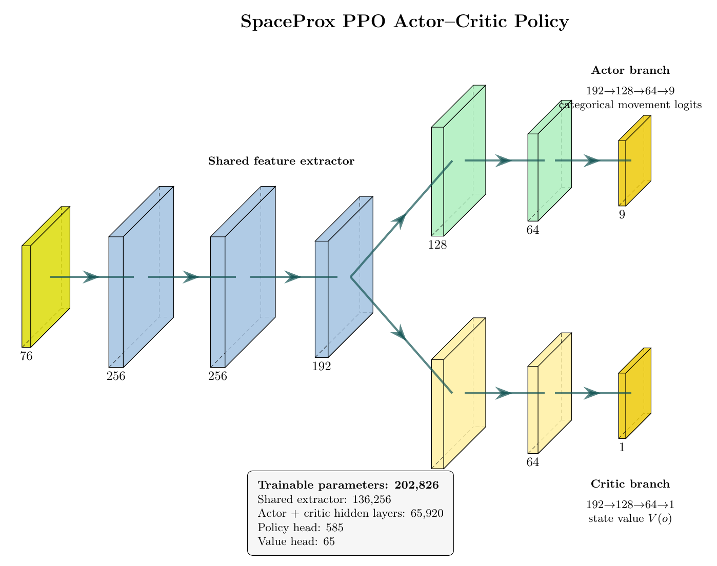
The shared feature extractor maps the 76-D observation through 76 -> 256 -> 256 -> 192, using Layer Normalization and SiLU after each linear layer. Layer Normalization follows Ba, Kiros, and Hinton (2016). The activation is SiLU, , which has also been studied explicitly for neural function approximation in reinforcement learning (Elfwing, Uchibe, and Doya, 2018). From the 192-D shared representation, the actor uses 192 -> 128 -> 64 -> 9 to produce categorical movement logits, while the critic uses 192 -> 128 -> 64 -> 1 to estimate .
The measured trainable-parameter breakdown is:
| Module | Trainable parameters |
|---|---|
| shared semantic feature extractor | 136,256 |
| actor + critic MLP extractor | 65,920 |
| 9-action output layer | 585 |
| value output layer | 65 |
| total | 202,826 |
This model is intentionally much smaller than a raw-pixel CNN. The point is not to win a parameter-count contest. The point is to place learning capacity where the experiment has enough interaction data to train it.
15. PPO training configuration
The controlled training configuration is:
learning_rate = 5.0e-4
n_steps = 128
batch_size = 64
n_epochs = 8
gamma = 0.990
gae_lambda = 0.95
clip_range = 0.20
ent_coef = 0.0002
vf_coef = 0.50
max_grad_norm = 0.50
target_kl = 0.030
With one environment, every complete PPO rollout contains 128 new game interactions. A full eight-epoch optimization with minibatches of 64 performs:
minibatch optimizer steps, unless the target-KL early-stop condition shortens the cycle. In Stable-Baselines3 the check is performed on each minibatch and stops the remaining epochs when the approximate KL exceeds 1.5 * target_kl; with target_kl = 0.03, that check is approximately 0.045.
Because early stopping can make the number of optimizer epochs per rollout vary, the experiment does not infer completed PPO cycles by simply dividing an internal epoch counter by eight. The snapshot callback counts actual completed optimization cycles and records them in a per-run manifest.
16. Backpropagation and gradient clipping
For each trainable parameter , gradient descent performs the conceptual update:
with learning rate .
Before the optimizer step, PyTorch rescales the aggregate gradient when its Euclidean norm exceeds 0.5. The post-clipping gradient therefore satisfies:
This does not make RL magically stable; it limits one class of destructive update where an unusually large minibatch gradient would otherwise move the network too far in one optimizer step.
17. What one environment step actually does
The full data path for one decision is:
1. Current screenshot-derived 76-D observation enters the neural policy.
2. Actor samples or argmaxes one of 9 movement actions.
3. Visual controller selects the nearest rendered enemy when one is visible.
4. Previous/current components estimate target motion.
5. Intercept equation chooses a cursor point.
6. Wrapper holds the corresponding WASD keys.
7. If a valid visual target exists, the low-level controller aims and holds Space automatically.
8. Game advances for ~80 ms.
9. PrintWindow captures the next rendered frame.
10. CV extracts new geometry and eight directional wall-clearance rays.
11. Public title supplies score/HP telemetry.
12. Reward and termination are calculated.
13. Transition enters PPO's rollout buffer.
After 128 such transitions, GAE and return targets are computed and the rollout is optimized for up to eight epochs.
18. Checkpoint Accounting and Training Data
This is one of the easiest places to write a technically misleading RL article.
Suppose a wall-clock stop fires after 2,514 environment interactions while the PPO rollout size is 128. Some final interactions can sit in an incomplete rollout that never reaches train(). A checkpoint saved at process exit can therefore contain a larger num_timesteps counter even though its neural weights are identical to an earlier optimized model.
The final trainer records both:
recorded_interactions
optimized_transitions
partial_rollout_interactions
completed_ppo_cycles
optimizer_epochs_total
last_optimized_model_path
Evaluation uses the last fully optimized snapshot rather than assuming the file with the largest timestep metadata necessarily contains newer weights.
Each run also gets its own checkpoint directory, epoch CSV, monitor log, snapshot manifest, and summary JSON. Reusing a run name is rejected instead of silently appending new data to an old experiment.
19. How I decide whether the agent actually learned
Training reward is not enough. A policy can collect score for the wrong behavioral reason, and RL curves are especially easy to cherry-pick. Henderson et al. (2018) discuss how variance and experimental methodology can make deep-RL results hard to reproduce; Machado et al. (2018) make a similar point in the game-evaluation context. More recent work makes the same warning quantitatively: few-run deep-RL comparisons need uncertainty-aware statistics (Agarwal et al., 2021), and careful empirical design is itself a substantial part of RL methodology (Patterson et al., 2024).
I therefore use several separate checks.
19.1. Training trajectories
Monitor logs preserve completed-life score, shaped return, and episode length. These describe what happened during on-policy training, but they are not held-out final evaluation.
19.2. Optimizer diagnostics
For every inner PPO epoch I log:
policy loss
value loss
entropy loss
approximate KL
clip fraction
total loss
learning rate
model timestep boundary
Entropy is interpreted against , not in isolation.
19.3. Deterministic behavior probe
A fixed-length probe records:
movement counts
number of unique movement actions
fraction of steps where a visual target was automatically engaged
player-detection fraction
policy entropy
maximum action probability
player x/y coverage
corner occupancy
stagnation fraction
blocked-motion fraction
low-clearance-action fraction
score / HP
completed episodes
This catches a failure that average training score can hide: an almost-uniform stochastic policy may look varied while training but collapse to one deterministic argmax action at deployment.
19.4. Multi-episode evaluation
The final claim should come from a fixed protocol over multiple evaluation episodes, reported separately for deterministic and stochastic action selection when both are interesting. A single lucky high-score run is evidence that something happened, not an estimate of expected performance.
19.5. Multiple seeds
One seed is a development experiment, not a strong statistical claim. A publication- quality result should repeat the final configuration over multiple seeds and report dispersion, not just the best run.
20. Experimental results
20.1. Hardware and software
| Item | Measured / configured value |
|---|---|
| GPU | NVIDIA GeForce RTX 4060 Laptop GPU |
| PyTorch | 2.11.0+cu128 |
| CUDA runtime | 12.8 |
| Stable-Baselines3 | 2.9.0 during the reported experiment |
| policy parameters | 202,826 |
| policy observation | 76 screenshot-derived / short-history float features |
| action space | Discrete(9) movement; visual combat controller auto-aims/fires |
| nominal action interval | 0.080 s |
20.2. Validated deployed checkpoint
The checkpoint I actually deploy comes from a five-minute training run with seed 41. I kept it because its deterministic movement probe passed the wall and stagnation checks described below.
| Measurement | Value |
|---|---|
| wall-clock training | 300.281 s |
| recorded environment interactions | 2,514 |
| transitions in completed optimized rollouts | 2,432 |
| partial-rollout interactions at stop | 82 |
| completed PPO rollout/update cycles | 19 |
| optimizer epochs completed | 148 |
| trainable parameters | 202,826 |
| seed | 41 |
The authoritative learned checkpoint is the last fully optimized snapshot, not the process-exit file with the larger timestep counter:
checkpoints/final/spaceprox_final_seed41_20260919_192039/
  optimized/spaceprox_ppo_cycle_0019_2432_steps.zip
No life ended during that five-minute training segment, so there is no completed training-episode average to report for this run.
20.3. Extended 30-minute training
I then repeated the same configuration for a full 30-minute wall-clock budget. This run is useful because 113 PPO rollouts give a much clearer view of the optimization dynamics than the short gate.
| Measurement | Value |
|---|---|
| wall-clock training | 1,800.328 s |
| recorded environment interactions | 14,560 |
| transitions in completed optimized rollouts | 14,464 |
| partial-rollout interactions at stop | 96 |
| completed PPO rollout/update cycles | 113 |
| optimizer epochs completed | 632 |
| completed training episodes | 1 |
| completed episode score | 89,600 |
| completed episode length | 2,889 steps |
| trainable parameters | 202,826 |
| seed | 41 |
The longer run was not automatically promoted just because it trained for more time. I evaluated its final fully optimized checkpoint separately.
These optimizer diagnostics answer different questions:
| Metric | Simple meaning |
|---|---|
| policy entropy | how uncertain the movement policy is |
| policy loss | the PPO surrogate objective used to improve the actor; its magnitude is an optimization diagnostic, not a gameplay score or direct measure of policy change |
| critic loss | how wrong the critic's future-reward prediction is |
| approximate KL | how far the updated policy moved from the policy that collected the rollout |
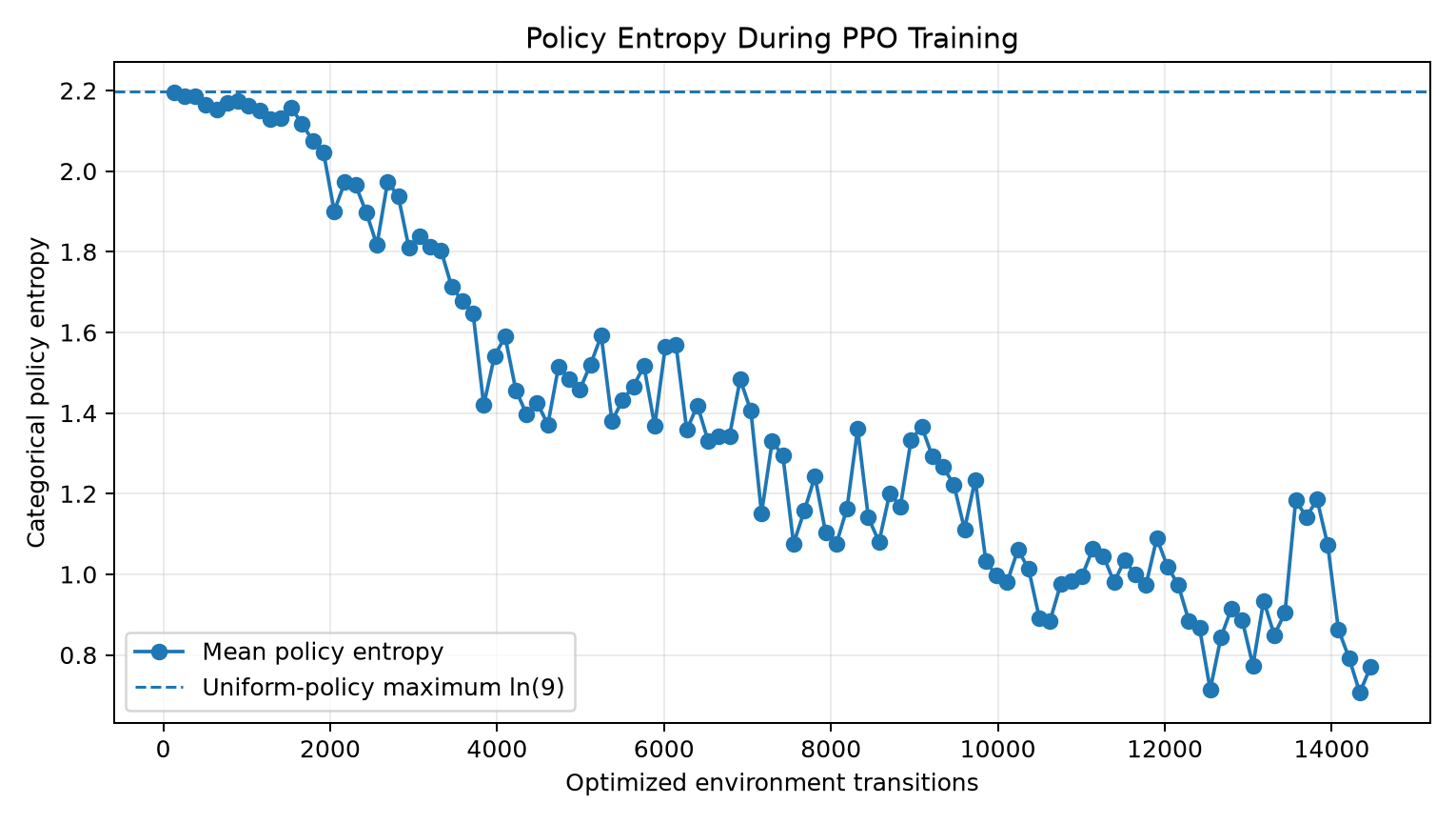
The first rollout is almost uniform at 2.19539 entropy, close to the nine-action maximum . By the final optimized rollout entropy has fallen to 0.76998, about 35.0% of the maximum. In plain language, the policy became much more decisive about which movement actions it preferred.
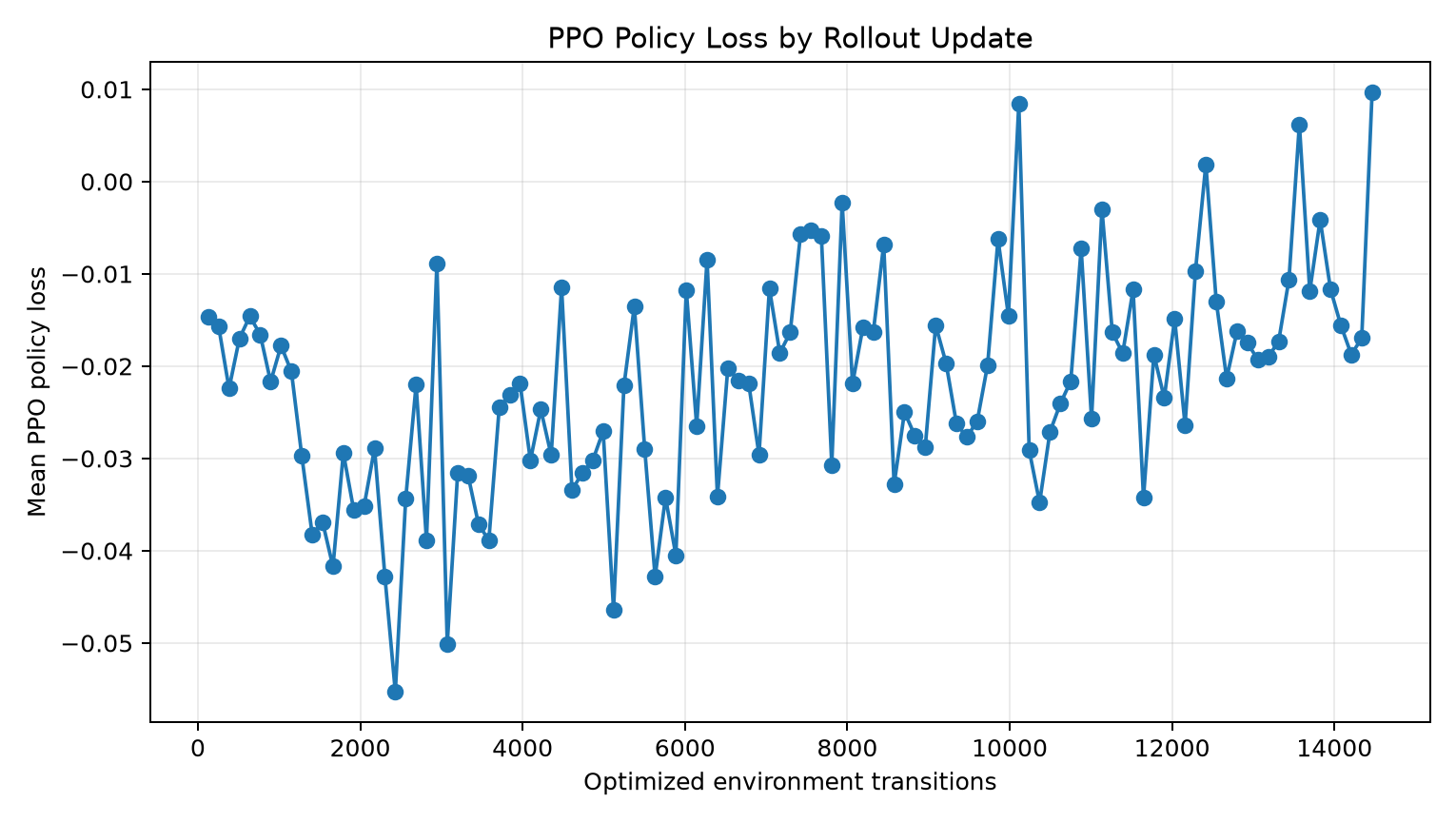
Policy loss is the clipped PPO surrogate objective used to update the actor. Its absolute value is not a gameplay score and it is not a direct measurement of how far the policy moved. It is also not expected to decrease smoothly like a supervised validation loss.
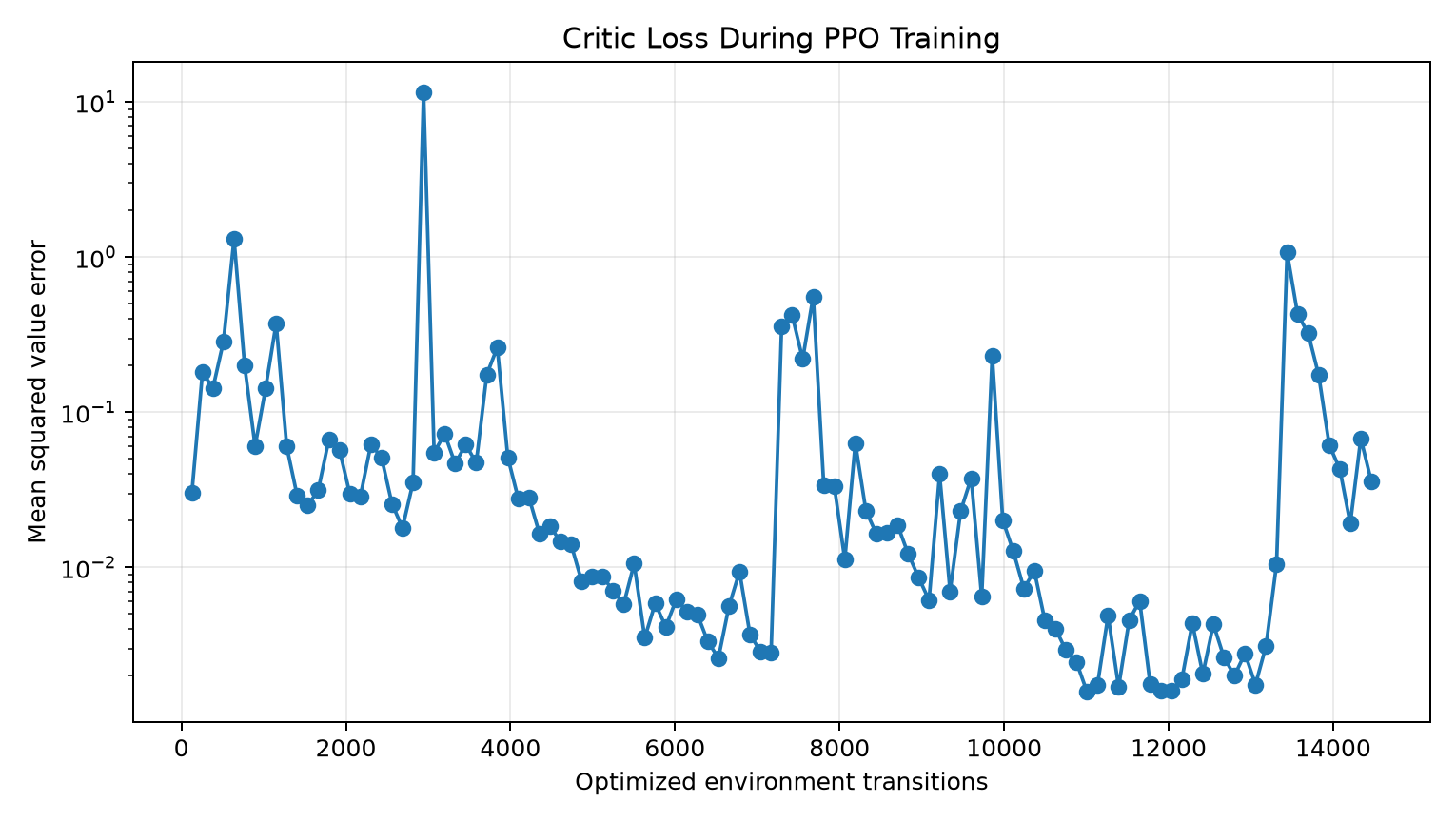
Critic loss is the value-prediction error. The figure uses a logarithmic vertical scale because a few large errors would otherwise flatten almost all of the ordinary updates against zero. Spikes mean some rollouts were harder for the critic to predict; a spike by itself does not prove that the movement policy got worse.
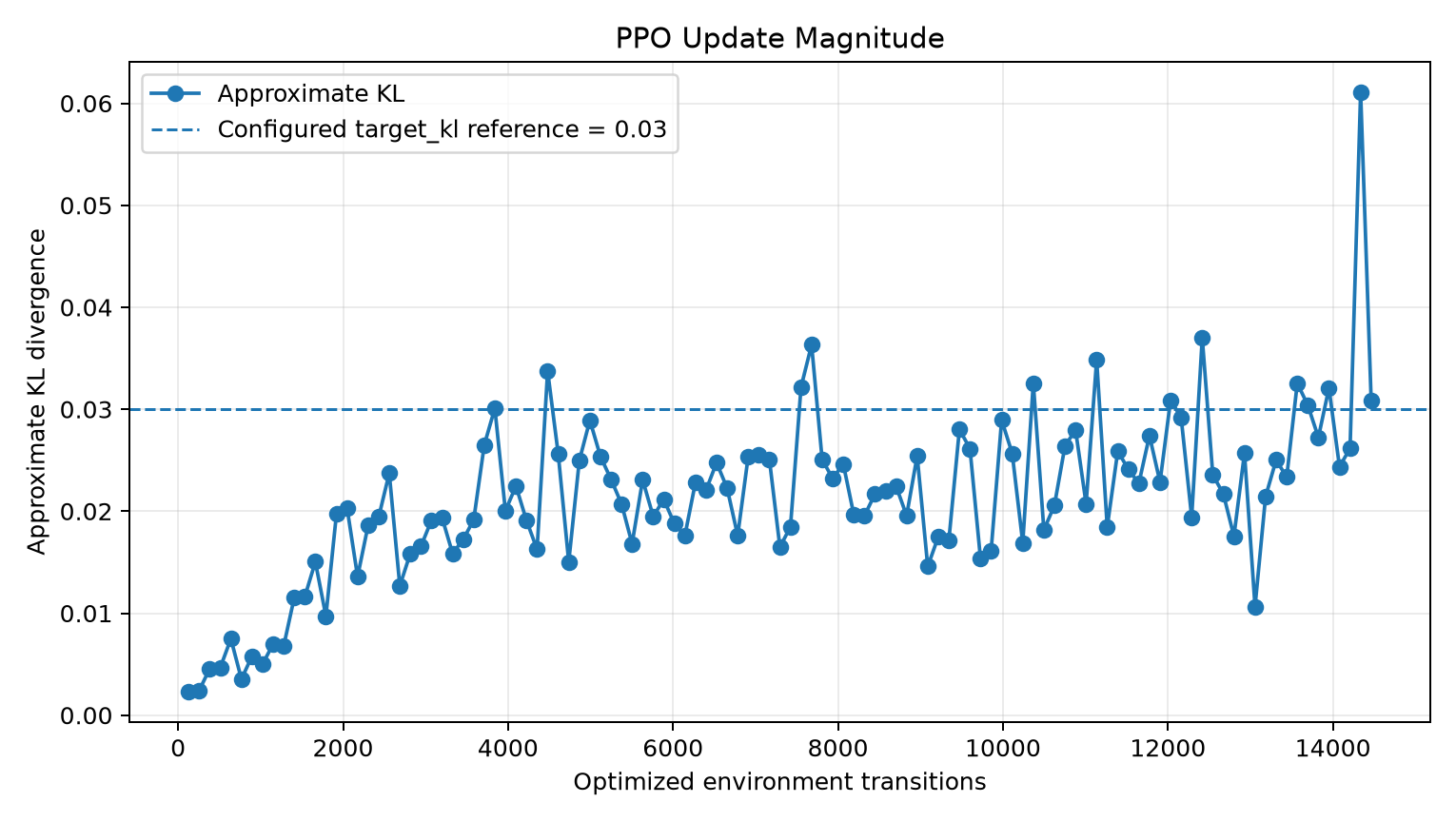
Approximate KL measures how far an update moved the policy. The dashed 0.03 line is only the configured target_kl reference for the rollout-level averages shown in the figure. Stable-Baselines3 performs early stopping on individual minibatches, not on these plotted rollout averages. The final rollout average is about 0.03085 and that rollout completed only three optimizer epochs because a minibatch triggered the KL early-stop guard.
The final 30-minute checkpoint was then tested for 300 deterministic steps:
| Probe statistic | 30-minute checkpoint |
|---|---|
| movement actions used | 4 (W, D, W+A, S+A) |
| dominant movement share | 58.0% |
| visual target automatically engaged | 88.7% of steps |
| player detection | 100% of steps |
| mean policy entropy | 0.67215 |
| mean maximum action probability | 0.7396 |
| blocked movement | 6.0% |
| stagnation | 0.67% |
| corner occupancy | 0% |
| selected direction with <30% clearance | 3.33% |
| score at end of probe | 5,150 |
| final / minimum HP | 60 |
The long-run policy is clearly not random. It is much more confident and still uses multiple movement actions. However, it also spent 6% of the probe blocked by a wall and lost substantially more HP than the deployed checkpoint did in its validation. I therefore did not replace the deployed model with the last 30-minute checkpoint. More gradient updates made the policy more confident, but not monotonically better at the behavior I care about.
This is also why checkpoint selection is based on a behavior test rather than simply choosing the file with the largest timestep count.
20.4. Deterministic behavior of the deployed checkpoint
The short-run gate was followed by a 300-step deterministic probe and then a stricter 1,000-step deterministic sanity run. This matters because the earlier wall-stuck failure only became obvious when deterministic argmax was watched over time.
| Probe statistic | Measured value |
|---|---|
| deterministic steps | 1,000 |
| movement actions used | 4 (W, W+A, S+A, S+D) |
| dominant movement share | 41.0% |
| visual target automatically engaged | 88.8% of steps |
| player detection | 100% of steps |
| mean policy entropy | 2.02344 |
| maximum possible entropy | 2.19722 |
| entropy / maximum | 92.09% |
| mean maximum action probability | 0.2331 |
| player x range | 437.84 to 919.59 px |
| player y range | 197.38 to 578.00 px |
| blocked movement | 0% |
| stagnation | 0% |
| corner occupancy | 0.2% |
| selected direction with <30% clearance | 9.4% |
| score at end of probe | 10,250 |
| final HP | 92 |
| minimum HP observed | 92 |
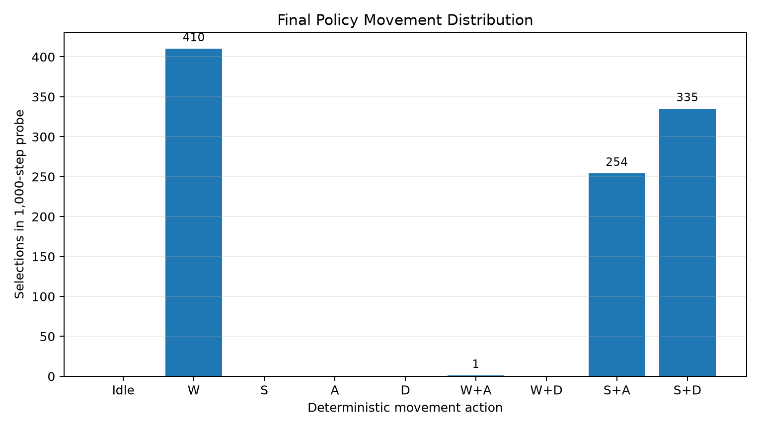
The 300-step gate already used three movement actions with zero blocked/stagnant steps; the 1,000-step run preserved that behavior and expanded to four actions. Most importantly, the policy did not return to the old failure mode of holding W against a wall. The player traversed hundreds of pixels in both axes while the low-level aiming controller remained active.
Using four actions is not, by itself, evidence of intelligent control. The useful observation is the combination of state-dependent action changes with zero measured blocked/stagnant steps, broad spatial coverage, low corner occupancy and preserved HP during the same fixed-length probe.
This does not prove the optimal movement strategy has been learned. It does establish the narrower engineering claim I care about here: the deterministic deployed policy became state-dependent enough to avoid the measured fixed-direction/wall-stuck degeneracy under a substantially longer probe.
Before training
The difference is easier to appreciate visually. Before training, I first used a deliberately simple control baseline to verify that capture and input were working. It could do exactly the wrong thing: keep an unhelpful heading and fire straight into a wall while enemies were visible elsewhere in the arena.
This is only a visual baseline for the external control loop. It is not evidence that PPO later learned the aim. In the final design, target selection, intercept aiming, and firing are deterministic; PPO learns the movement policy.
After training
With the validated controller, movement is no longer dominated by the old wall-stuck behavior, while the deterministic visual combat layer keeps the player aligned with a useful target. This frame is from the final deployed setup.
20.5. What the result supports
The current controller is a working black-box controller with effective visual combat and non-degenerate learned movement. I still do not call the game solved. Both the deployed checkpoint and the extended run use one seed, and the fixed-length behavior probes are not a substitute for a multi-seed, fixed-episode evaluation protocol. A stronger research claim should repeat the configuration over several seeds and report dispersion rather than promoting the best single run.
More specifically, the present evidence supports the claim that this saved policy learned non-degenerate, state-dependent movement and avoided the previously measured wall-stuck failure in a 1,000-step deterministic probe. It does not establish a statistically significant improvement in expected score or survival over random or zero-update movement, because a matched baseline distribution and multiple training seeds have not been measured. I keep that distinction explicit rather than treating healthy optimizer curves as proof of task performance.
21. Failure modes and limitations
21.1. The perception system is hand engineered
The neural policy does not learn its own detector. Green/red thresholding and connected-component rules are domain knowledge. This is a feature for sample efficiency and a limitation for generality.
21.2. The hierarchy changes the learning problem
PPO is not learning raw cursor aim. The low-level controller handles visual target selection and interception. Therefore this experiment should be compared to hybrid or hierarchical control, not described as pure end-to-end pixel RL.
21.3. Reward shaping can bias the optimum
The practical penalties are not proven policy-invariant. Ng et al. (1999) is exactly why I state this explicitly rather than calling every shaping term theoretically safe.
21.4. Title telemetry is temporally coarse
Score and HP in the title refresh more slowly than the 80 ms action loop. A score or damage event can therefore be assigned to a nearby later environment transition. Visual GAME OVER detection fixes terminal latency but does not eliminate all reward credit delay.
21.5. One game process limits throughput
The most successful deep-RL systems rely on huge experience budgets or parallel actors (Mnih et al., 2016; Berner et al., 2019; Vinyals et al., 2019). Here, single-instance throughput is part of the challenge.
21.6. Windows input is a physical interface
Keyboard state and cursor position are global OS resources. Running two controllers at the same time would contaminate both experiments. A valid run therefore checks that only one trainer and one game process are active.
21.7. Deterministic CV can still fail
Color changes, overlays, resolution changes, or a redesigned HUD can break a threshold detector. The black-box boundary is preserved, but robustness to visual domain shift is not solved.
21.8. Reproducibility is not the same as determinism
The seed, code, checkpoints and metrics are preserved, but the game is a real-time Windows process and scheduling/capture timing can vary. Exact bit-for-bit trajectory replay should not be assumed.
21.9. Intercept timing is approximate
Enemy velocity for the low-level lead calculation is estimated from displacement between captured frames and divided by the configured 80 ms control interval. The actual capture-to-capture wall time also includes perception and operating-system scheduling jitter, so the inferred velocity and projectile intercept are approximate. This does not affect the PPO mathematics, but it is a limitation of the engineered combat controller and another reason not to interpret its aiming quality as learned movement performance.
22. What I would test next
The most useful follow-up experiments are controlled ablations, not arbitrary model growth.
- Multiple seeds. Repeat the final hyperparameters and report mean/median and
- Reward ablation. Remove wall-clearance, blocked/stagnation and danger terms one at a time.
- Perception ablation. Compare the 76-D semantic policy against a learned visual
- Action abstraction ablation. Compare hierarchical targeting against direct
- Faster telemetry. Add an external synchronized measurement path without
- Parallel isolated processes. If Windows input can be virtualized per instance,
- Modern visual-RL baselines. With enough interaction budget, compare ideas from
standard deviation.
encoder at the same interaction budget.
learned aim only if the interaction budget is large enough.
reading game memory, or derive more reward events from pixels.
parallel actors would change the sample-budget problem completely.
CURL/DrQ/DrQ-v2 rather than assuming PPO + hand perception is universally best.
23. Source Code
The complete game, RL code, trained model, install script and run scripts are available in the public repository:
24. References
- Rishabh Agarwal, Max Schwarzer, Pablo Samuel Castro, Aaron Courville, and Marc G. Bellemare. "Deep Reinforcement Learning at the Edge of the Statistical Precipice." NeurIPS 2021. https://arxiv.org/abs/2108.13264
- Jimmy Lei Ba, Jamie Ryan Kiros, and Geoffrey E. Hinton. "Layer Normalization." arXiv:1607.06450, 2016.
- Pierre-Luc Bacon, Jean Harb, and Doina Precup. "The Option-Critic Architecture." AAAI 2017, pp. 1726-1734. DOI: 10.1609/aaai.v31i1.10916.
- Adrià Puigdomènech Badia et al. "Agent57: Outperforming the Atari Human Benchmark." arXiv:2003.13350, 2020.
- Marc G. Bellemare, Yavar Naddaf, Joel Veness, and Michael Bowling. "The Arcade Learning Environment: An Evaluation Platform for General Agents." Journal of Artificial Intelligence Research 47:253-279, 2013. DOI: 10.1613/JAIR.3912.
- Christopher Berner et al. "Dota 2 with Large Scale Deep Reinforcement Learning." arXiv:1912.06680, 2019.
- Stefan Elfwing, Eiji Uchibe, and Kenji Doya. "Sigmoid-weighted linear units for neural network function approximation in reinforcement learning." Neural Networks 107:3-11, 2018. DOI: 10.1016/j.neunet.2017.12.012.
- Lasse Espeholt, Hubert Soyer, Remi Munos, Karen Simonyan, Vlad Mnih, Tom Ward, Yotam Doron, Vlad Firoiu, Tim Harley, Iain Dunning, Shane Legg, and Koray Kavukcuoglu. "IMPALA: Scalable Distributed Deep-RL with Importance Weighted Actor-Learner Architectures." ICML 2018, PMLR 80:1407-1416. https://proceedings.mlr.press/v80/espeholt18a.html
- David Ha and Jürgen Schmidhuber. "World Models." arXiv:1803.10122, 2018. https://arxiv.org/abs/1803.10122
- Danijar Hafner, Timothy Lillicrap, Mohammad Norouzi, and Jimmy Ba. "Mastering Atari with Discrete World Models." ICLR 2021. https://arxiv.org/abs/2010.02193
- Danijar Hafner, Jurgis Pasukonis, Jimmy Ba, and Timothy Lillicrap. "Mastering diverse control tasks through world models." Nature 640:647-653, 2025. DOI: 10.1038/s41586-025-08744-2.
- Peter Henderson, Riashat Islam, Philip Bachman, Joelle Pineau, Doina Precup, and David Meger. "Deep Reinforcement Learning That Matters." AAAI 2018. DOI: 10.1609/aaai.v32i1.11694.
- Matteo Hessel et al. "Rainbow: Combining Improvements in Deep Reinforcement Learning." AAAI 2018. DOI: 10.1609/aaai.v32i1.11796.
- Seth Hutchinson, Gregory D. Hager, and Peter I. Corke. "A Tutorial on Visual Servo Control." IEEE Transactions on Robotics and Automation 12(5):651-670, 1996. DOI: 10.1109/70.538972.
- Max Jaderberg et al. "Human-level performance in 3D multiplayer games with population-based reinforcement learning." Science 364(6443):859-865, 2019. DOI: 10.1126/science.aau6249.
- Leslie Pack Kaelbling, Michael L. Littman, and Anthony R. Cassandra. "Planning and acting in partially observable stochastic domains." Artificial Intelligence 101(1-2):99-134, 1998. DOI: 10.1016/S0004-3702(98)00023-X.
- Ilya Kostrikov, Denis Yarats, and Rob Fergus. "Image Augmentation Is All You Need: Regularizing Deep Reinforcement Learning from Pixels." arXiv:2004.13649, 2020.
- Tejas D. Kulkarni, Karthik R. Narasimhan, Ardavan Saeedi, and Joshua B. Tenenbaum. "Hierarchical Deep Reinforcement Learning: Integrating Temporal Abstraction and Intrinsic Motivation." NeurIPS 2016.
- Michael Laskin, Aravind Srinivas, and Pieter Abbeel. "CURL: Contrastive Unsupervised Representations for Reinforcement Learning." ICML 2020, PMLR 119:5639-5650.
- Sergey Levine, Chelsea Finn, Trevor Darrell, and Pieter Abbeel. "End-to-End Training of Deep Visuomotor Policies." Journal of Machine Learning Research 17(39):1-40, 2016. https://jmlr.org/papers/v17/15-522.html
- Marlos C. Machado, Marc G. Bellemare, Erik Talvitie, Joel Veness, Matthew Hausknecht, and Michael Bowling. "Revisiting the Arcade Learning Environment: Evaluation Protocols and Open Problems for General Agents." Journal of Artificial Intelligence Research 61:523-562, 2018.
- Volodymyr Mnih, Koray Kavukcuoglu, David Silver, Alex Graves, Ioannis Antonoglou, Daan Wierstra, and Martin Riedmiller. "Playing Atari with Deep Reinforcement Learning." arXiv:1312.5602, 2013.
- Volodymyr Mnih et al. "Human-level control through deep reinforcement learning." Nature 518:529-533, 2015. DOI: 10.1038/nature14236.
- Volodymyr Mnih, Adrià Puigdomènech Badia, Mehdi Mirza, Alex Graves, Timothy Lillicrap, Tim Harley, David Silver, and Koray Kavukcuoglu. "Asynchronous Methods for Deep Reinforcement Learning." ICML 2016, PMLR 48:1928-1937.
- Andrew Y. Ng, Daishi Harada, and Stuart Russell. "Policy Invariance Under Reward Transformations: Theory and Application to Reward Shaping." ICML 1999, pp. 278-287.
- Andrew Patterson, Samuel Neumann, Martha White, and Adam White. "Empirical Design in Reinforcement Learning." Journal of Machine Learning Research 25(318):1-63, 2024. https://www.jmlr.org/papers/v25/23-0183.html
- Aleksei Petrenko, Zhehui Huang, Tushar Kumar, Gaurav S. Sukhatme, and Vladlen Koltun. "Sample Factory: Egocentric 3D Control from Pixels at 100000 FPS with Asynchronous Reinforcement Learning." ICML 2020, PMLR 119:7652-7662. https://proceedings.mlr.press/v119/petrenko20a.html
- Antonin Raffin, Ashley Hill, Adam Gleave, Anssi Kanervisto, Maximilian Ernestus, and Noah Dormann. "Stable-Baselines3: Reliable Reinforcement Learning Implementations." Journal of Machine Learning Research 22(268):1-8, 2021. https://jmlr.org/papers/v22/20-1364.html
- John Schulman, Philipp Moritz, Sergey Levine, Michael Jordan, and Pieter Abbeel. "High-Dimensional Continuous Control Using Generalized Advantage Estimation." arXiv:1506.02438, 2015. https://arxiv.org/abs/1506.02438
- John Schulman, Filip Wolski, Prafulla Dhariwal, Alec Radford, and Oleg Klimov. "Proximal Policy Optimization Algorithms." arXiv:1707.06347, 2017. https://arxiv.org/abs/1707.06347
- John Schulman, Sergey Levine, Pieter Abbeel, Michael Jordan, and Philipp Moritz. "Trust Region Policy Optimization." ICML 2015, PMLR 37:1889-1897. https://proceedings.mlr.press/v37/schulman15.html
- Ramanan Sekar, Oleh Rybkin, Kostas Daniilidis, Pieter Abbeel, Danijar Hafner, and Deepak Pathak. "Planning to Explore via Self-Supervised World Models." ICML 2020, PMLR 119:8583-8592. https://proceedings.mlr.press/v119/sekar20a.html
- Richard S. Sutton and Andrew G. Barto. Reinforcement Learning: An Introduction, 2nd ed. MIT Press, 2018. http://incompleteideas.net/book/the-book-2nd.html
- Richard S. Sutton, David McAllester, Satinder Singh, and Yishay Mansour. "Policy Gradient Methods for Reinforcement Learning with Function Approximation." NeurIPS 1999, pp. 1057-1063. https://papers.nips.cc/paper/1713-policy-gradient-methods-for-reinforcement-learning-with-function-approximation
- Richard S. Sutton, Doina Precup, and Satinder Singh. "Between MDPs and semi-MDPs: A framework for temporal abstraction in reinforcement learning." Artificial Intelligence 112(1-2):181-211, 1999. DOI: 10.1016/S0004-3702(99)00052-1.
- Alexander Sasha Vezhnevets et al. "FeUdal Networks for Hierarchical Reinforcement Learning." ICML 2017, PMLR 70:3540-3549.
- Oriol Vinyals et al. "Grandmaster level in StarCraft II using multi-agent reinforcement learning." Nature 575:350-354, 2019. DOI: 10.1038/s41586-019-1724-z.
- Denis Yarats, Rob Fergus, Alessandro Lazaric, and Lerrel Pinto. "Mastering Visual Continuous Control: Improved Data-Augmented Reinforcement Learning." arXiv:2107.09645, 2021.
Closing note
What I like about this experiment is not that it reproduces Atari, Dota, or AlphaStar on a laptop. It obviously does not. It makes the interface problem visible. Once the game stops being a cooperative simulator, reinforcement learning becomes a systems project: sensing, timing, action abstraction, process lifecycle, Windows input, reward latency, experiment accounting, and only then neural optimization.